Density Functional Theory in Python Code (2D External Potential)
This note book follows the example as illustrate in the following link
Density Functinoal Theory in Python (1D)
First we need to import the plotting tools for 3D. There are many out there. Here I choose to use matplot3d
from mpl_toolkits.mplot3d import Axes3D
import numpy as np
import matplotlib.pyplot as plt
import seaborn as sns
%matplotlib inline
sns.set_style("white")
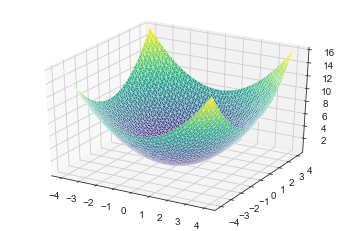
Below we create a 2D parabolic function and plotted out the 3D surface
n_grid=50
x=np.linspace(-4,4,n_grid)
y=np.linspace(-4,4,n_grid)
mesh = np.meshgrid(x, y)
xmesh, ymesh = mesh
zmesh = 0.5*(xmesh**2+ymesh**2)
xflat = xmesh.flatten()
yflat = ymesh.flatten()
zflat = zmesh.flatten()
fig = plt.figure()
ax = fig.gca(projection='3d')
ax.plot_trisurf(xflat, yflat, zflat, cmap=plt.cm.viridis, linewidth=0.2)
plt.show()
For two dimensional system, the Hamiltonian operator is
\begin{align} \hat{H} = -\frac{1}{2}(\nabla_x^2 + \nabla_y^2) \end{align} in atomic unit, where m = 1, and $\hbar$ = 1
We use finite difference to calculate the differntial
\begin{align}
h = x_{i+1} - x_{i} = y_{i+1}-y_{i}
D_x = \frac{Z_{i+1,j} - Z_{i,j}}{h}
D_y = \frac{Z_{i,j+1} - Z_{i,j}}{h}
\end{align}
However, two dimentional representation of function Z is very inconvienient. Here we flatten Z into one dimensional vector using numpy flatten function.
As a result, D_x and D_y become the kronecker product of the original D matrix in 1D space with the Identity Matrix.
\begin{align}
D_x = {D}\otimes{I}
D_y = {I}\otimes{D}
\end{align}
We can still calculate the second dirivitive by $D_x^2 = -D_xD_x^T$ and $D_y^2 = -D_yD_y^T$
h=x[1]-x[0]
D=-np.eye(n_grid)+np.diagflat(np.ones(n_grid-1),1)
D = D / h
Dx = np.kron(np.eye(n_grid), D)
Dy = np.kron(D, np.eye(n_grid))
Dx2 = Dx.dot(-Dx.T)
Dy2 = Dy.dot(-Dy.T)
Now we have the kinetic part of the $\hat{H}$, we can add the parabolic potential function Z to the Hamiltonian. And the final Hamiltonian is \begin{align} \hat{H} = -\frac{1}{2}(\nabla_x^2+\nabla_y^2) + \frac{1}{2}(x^2+y^2) \end{align}
Then we will obtain the $\hat{H}$ representation in coordinate basis and we can diagonalize the matrix and obtain the eigenvalues and eigenvectors. This can be done using numpy linear algebra package.
Z=np.diagflat(zflat)
eig_harm, psi_harm=np.linalg.eigh(-(Dx2+Dy2)/2+Z)
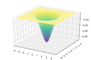
Now we have Eigenvalues (Energies!) and Eigenvectors (Orbitals!) we can plot them out. We will first plot out the lowest orbital.
fig = plt.figure()
ax = fig.gca(projection='3d')
ax.plot_trisurf(xflat,yflat,psi_harm[:,0],cmap=plt.cm.viridis, linewidth=0.2)
plt.show()
plt.contourf(x, y, psi_harm[:,0].reshape(n_grid,n_grid), 20, cmap='RdGy')
plt.colorbar()
print(eig_harm[0])
0.9983310783944462
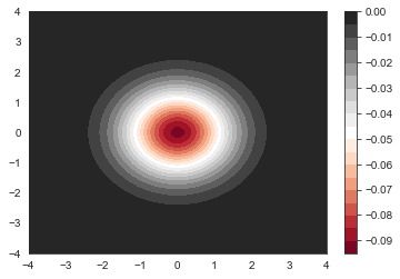
We can see that the lowest lying orbital does not have any node in it. That’s what we expected. It has a energy of 0.9983310783944462 (should be 1 because of rounding error and finite basis set used). Now let’s look into higher lying orbital start from 1.
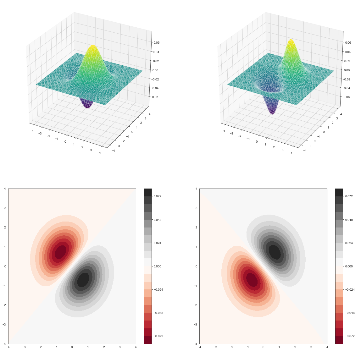
This orbtial has 1 node it it. That’s the first excited orbital (That’s also what we expected). It has a energy of 1.994985677390388 (Should be 2 exactly). Now let’s move to the second orbital.
Now we start to see something intresting. This orbital also have 1 node and energy of 1.9949856773903958 (should be 2) which is the same as the first orbital. In this case, the second orbital and first orbtial are degenerate
fig = plt.figure(figsize=(20,20))
ax = fig.add_subplot(2, 2, 1, projection='3d')
ax.plot_trisurf(xflat,yflat,psi_harm[:,1],cmap=plt.cm.viridis, linewidth=0.2)
ax = fig.add_subplot(2, 2, 2, projection='3d')
ax.plot_trisurf(xflat,yflat,psi_harm[:,2],cmap=plt.cm.viridis, linewidth=0.2)
ax = fig.add_subplot(2, 2, 3)
orb1=ax.contourf(x, y, psi_harm[:,1].reshape(n_grid,n_grid), 20, cmap='RdGy')
fig.colorbar(orb1, ax=ax)
ax = fig.add_subplot(2, 2, 4)
orb2=ax.contourf(x, y, psi_harm[:,2].reshape(n_grid,n_grid), 20, cmap='RdGy')
fig.colorbar(orb2, ax=ax)
plt.show()
print(eig_harm[1], eig_harm[2])
1.994985677390388 1.9949856773903958
Now let’s move to the third, fourth, fifth orbital. This three orbtials have very close energies. They are degenerate.
fig = plt.figure(figsize=(20,20))
ax = fig.add_subplot(2,3,1,projection='3d')
ax.plot_trisurf(xflat,yflat,psi_harm[:,3],cmap=plt.cm.viridis, linewidth=0.2)
ax = fig.add_subplot(2,3,2,projection='3d')
ax.plot_trisurf(xflat,yflat,psi_harm[:,4],cmap=plt.cm.viridis, linewidth=0.2)
ax = fig.add_subplot(2,3,3,projection='3d')
ax.plot_trisurf(xflat,yflat,psi_harm[:,5],cmap=plt.cm.viridis, linewidth=0.2)
ax = fig.add_subplot(2,3,4)
orb3=ax.contourf(x, y, psi_harm[:,3].reshape(n_grid,n_grid), 20, cmap='RdGy')
fig.colorbar(orb3,ax=ax)
ax = fig.add_subplot(2,3,5)
orb4=ax.contourf(x, y, psi_harm[:,4].reshape(n_grid,n_grid), 20, cmap='RdGy')
fig.colorbar(orb4,ax=ax)
ax = fig.add_subplot(2,3,6)
orb5=ax.contourf(x, y, psi_harm[:,5].reshape(n_grid,n_grid), 20, cmap='RdGy')
fig.colorbar(orb5,ax=ax)
print(eig_harm[3],eig_harm[4],eig_harm[5])
2.9882552654219587 2.988255265422003 2.9916402763863372
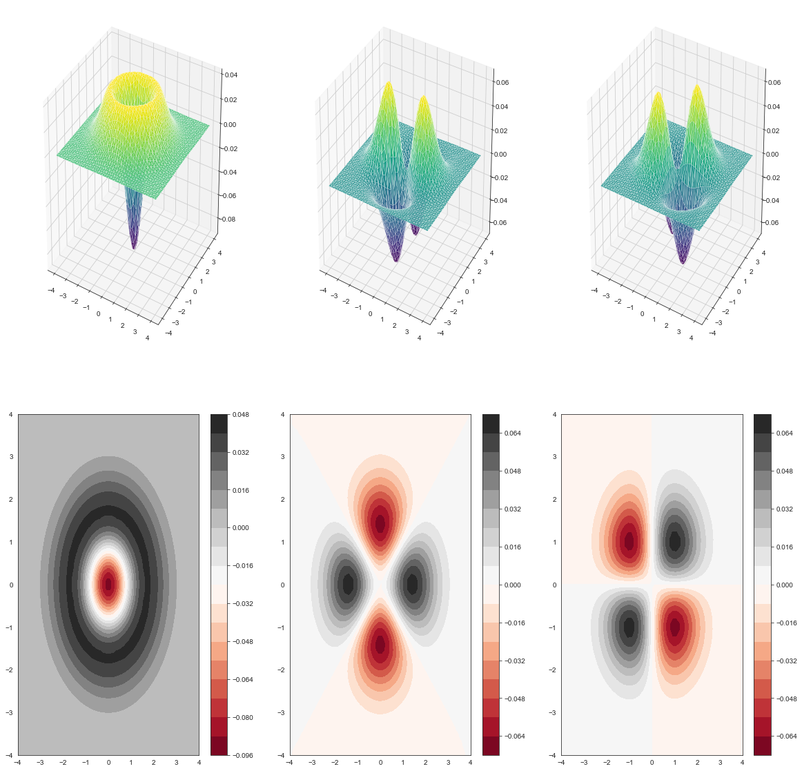
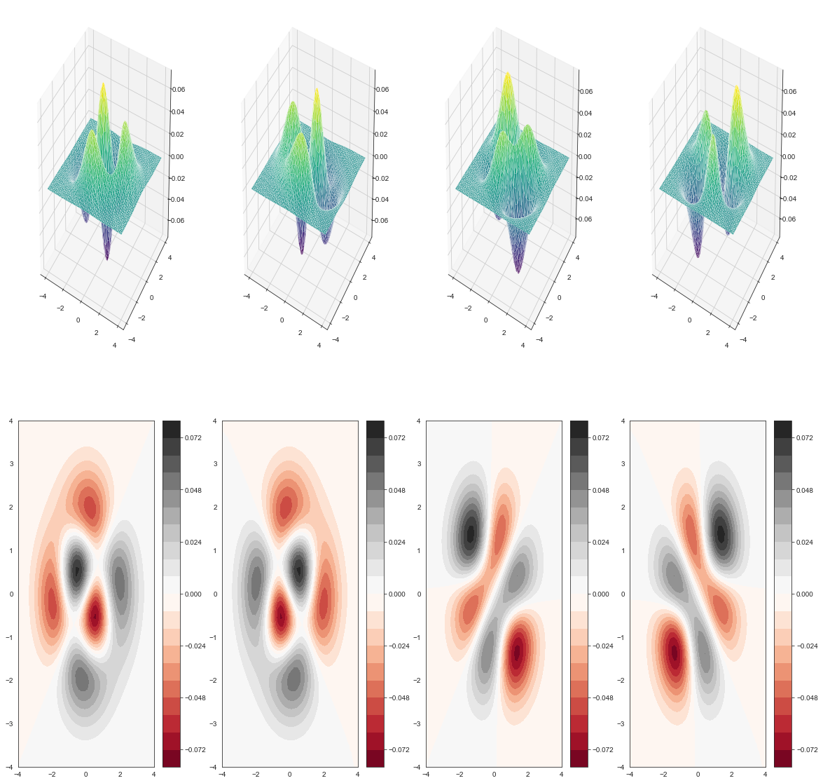
Now let’s see the sixth, seventh, eigth, nineth orbital.
fig = plt.figure(figsize=(20,20))
ax = fig.add_subplot(2,4,1,projection='3d')
ax.plot_trisurf(xflat,yflat,psi_harm[:,6],cmap=plt.cm.viridis, linewidth=0.2)
ax = fig.add_subplot(2,4,2,projection='3d')
ax.plot_trisurf(xflat,yflat,psi_harm[:,7],cmap=plt.cm.viridis, linewidth=0.2)
ax = fig.add_subplot(2,4,3,projection='3d')
ax.plot_trisurf(xflat,yflat,psi_harm[:,8],cmap=plt.cm.viridis, linewidth=0.2)
ax = fig.add_subplot(2,4,4,projection='3d')
ax.plot_trisurf(xflat,yflat,psi_harm[:,9],cmap=plt.cm.viridis, linewidth=0.2)
ax = fig.add_subplot(2,4,5)
orb6=ax.contourf(x, y, psi_harm[:,6].reshape(n_grid,n_grid), 20, cmap='RdGy')
fig.colorbar(orb6,ax=ax)
ax = fig.add_subplot(2,4,6)
orb7=ax.contourf(x, y, psi_harm[:,7].reshape(n_grid,n_grid), 20, cmap='RdGy')
fig.colorbar(orb7,ax=ax)
ax = fig.add_subplot(2,4,7)
orb8=ax.contourf(x, y, psi_harm[:,8].reshape(n_grid,n_grid), 20, cmap='RdGy')
fig.colorbar(orb8,ax=ax)
ax = fig.add_subplot(2,4,8)
orb9=ax.contourf(x, y, psi_harm[:,9].reshape(n_grid,n_grid), 20, cmap='RdGy')
fig.colorbar(orb9,ax=ax)
print(eig_harm[6],eig_harm[7],eig_harm[8],eig_harm[9])
3.977930246184832 3.9779302461848434 3.984909864417891 3.9849098644179026
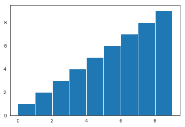
We can also plot the density of states for this 2D harmonic oscillator. The density of states is a linear function of energy.
plt.hist(eig_harm,bins=range(10))
(array([1., 2., 3., 4., 5., 6., 7., 8., 9.]),
 array([0, 1, 2, 3, 4, 5, 6, 7, 8, 9]),
 <a list of 9 Patch objects>)
For this harmonic oscillator, we can solve the Schrödinger’s Equation Excatly. The energy levels are \begin{align} E=(n_x+\frac{1}{2})\hbar\omega_x + (n_y+\frac{1}{2})\hbar\omega_y = (n_x + n_y + 1) \end{align} where $n_x$ and $n_y$ are the quantum numbers for the x and y directions, respectively. Since $\omega_x = \omega_y = 1$.The additional 1 is for Zero point energy. From this equation, we can easily obtain the degeneracy of level n as n + 1 as there are n + 1 solutions of ($n_x$,$n_y$) for $n_x+n_y=n$
The orbtial is
\begin{align}
\psi_{m,n}(x,y)= \psi_m(x)\psi_n(y)
\psi_m(x) = \frac{1}{\sqrt{2^mm!}}\pi^{-1/4}exp(-x^2/2)H_m(x)
\psi_n(y) = \frac{1}{\sqrt{2^nn!}}\pi^{-1/4}exp(-y^2/2)H_n(y)
\end{align}
where $H_n(x)$ is nth order Hermite Polynomials
If you look carefully at the node (zero point) of the wave function $\psi_{m,n}(x,y)$, you will notice that $\psi_{1,0}$ and $\psi_{0,1}$ has node $x=0$ and $y=0$,respectively. However, the orbital 1 and orbital2 we calculated have node of $x - y = 0$ and $x + y = 0$, respectively.
Acutally, our orbital 1 and 2 are linear combinations of $\psi_{1,0}$ and $\psi_{0,1}$
\begin{align}
orbital 1 = \frac{1}{\sqrt{2}}(\psi_{1,0}(x,y) - \psi_{0,1}(x,y))
orbital 2 = \frac{1}{\sqrt{2}}(\psi_{1,0}(x,y) + \psi_{0,1}(x,y))
\end{align}
We can do this linear combination without causing change in orbital energies since these orbitals are degenerated and these transformed orbitals are still the eigenvectors of the Hamiltonian.
Similarly,
\begin{align}
orbital 3 = \frac{1}{\sqrt{2}}(\psi_{2,0}(x,y) + \psi_{0,2}(x,y))
orbital 4 = \frac{1}{\sqrt{2}}(\psi_{2,0}(x,y) - \psi_{0,2}(x,y))
orbital 5 = \psi_{1,1}(x,y)
\end{align}
and
\begin{align}
orbital 6 = \frac{1}{2}(\psi_{3,0}(x,y) - \psi_{0,3}(x,y) - \psi_{2,1}(x,y) + \psi_{1,2}(x,y))
orbital 7 = \frac{1}{2}(\psi_{3,0}(x,y) + \psi_{0,3}(x,y) + \psi_{2,1}(x,y) + \psi_{1,2}(x,y))
orbital 8 = \frac{1}{2}(\psi_{3,0}(x,y) - \psi_{0,3}(x,y) + \psi_{2,1}(x,y) - \psi_{1,2}(x,y))
orbital 9 = \frac{1}{2}(\psi_{3,0}(x,y) + \psi_{0,3}(x,y) - \psi_{2,1}(x,y) - \psi_{1,2}(x,y))
\end{align}
Now Add More than One electrons
All the above analysis only considers the one electron in the orbtial (1 Body problem). In reality there are many electrons fill the orbitals. Now let’s start adding electrons to the orbitals.
#integral
def integral(x, y, psi, axis = 0):
    dx = x[1] - x[0]
    dy = y[1] - y[0]
    return np.sum(psi*dx*dy, axis = axis)
num_electrons = 12
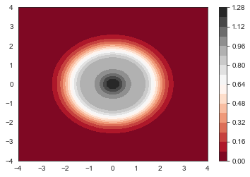
Now let’s calculate the ground state electron density $n(x,y)$
def get_nxy(num_electrons, psi, x, y):
    # normalization
    I=integral(x,y, psi**2,axis=0)
    normed_psi=psi/np.sqrt(I)

    # occupation num
    fn=[2 for _ in range(num_electrons//2)]
    if num_electrons % 2:
        fn.append(1)

    # density
    res=np.zeros_like(normed_psi[:,0])
    for ne, psi  in zip(fn,normed_psi.T):
        res += ne*(psi**2)
    return res
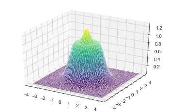
fig = plt.figure()
ax = fig.gca(projection='3d')
ax.plot_trisurf(xflat,yflat,get_nxy(num_electrons, psi_harm, x, y),cmap=plt.cm.viridis, linewidth=0.2)
plt.show()
plt.contourf(x, y, get_nxy(num_electrons, psi_harm, x, y).reshape(n_grid,n_grid), 20, cmap='RdGy')
plt.colorbar()
plt.show()
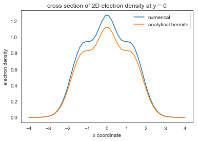
plt.plot(x,get_nxy(num_electrons, psi_harm, x, y).reshape(n_grid, n_grid)[:,n_grid//2])
plt.xlabel('x coordinate')
plt.ylabel('electron density')
plt.title('cross section of 2D electron density at y = 0')
plt.plot(x, (1+1/2*4*x**2+1/8*(4*x**2-2)**2+1/8*2**2)*np.exp(-x**2)*np.pi**(-1/2))
plt.legend(('numerical', 'analytical hermite'),loc='upper right')
<matplotlib.legend.Legend at 0x13c471780>
Energy Exchange
Consider the exchange functional in the LDA: For now ignore the correlation functional for simplicity: \begin{align} E_{X}^{LDA}[n(x,y)] = -\frac{3}{4}(\frac{3}{\pi})^{\frac{1}{3}}\int{n(x,y)^{\frac{4}{3}}}dxdy \end{align}
The potential is given by the functional derivative of the exchange energy $E_{x}^{LDA}$ with respect to the density $n(x,y)$
\begin{align} v_{x}^{LDA} = = -(\frac{3}{\pi})^{\frac{1}{3}}n(x,y)^{\frac{1}{3}} \end{align}
def get_exchange(nxy,x,y):
    energy=-3/4*(3/np.pi)**(1/3)*integral(x,y,nxy**(4/3))
    potential=-(3/np.pi)**(1/3)*nxy**(1/3)
    return energy, potential
Coumlobic potential
Electrostatic or Hartree energy \begin{align} E_{hartree}[n] = 1/2 \int\int{\frac{n(x’,y’)n(x,y)}{\sqrt{(x-x’)^2+(y-y’)^2}}}dxdydx’dy’ \end{align}
The potential is again the functional derivative of $E_{hartree}$ with respect to $n(x,y)$ \begin{align} v_{hartree}[n] = \int{\frac{n(x,y)}{\sqrt{(x-x’)^2+(y-y’)^2}}}dx’dy’ \end{align}
def get_hatree(nxy,x,y,xflat,yflat,eps=1e-7):
    hx=x[1]-x[0]
    hy=y[1]-y[0]
    energy=1/2*np.sum(nxy[None,:]*nxy[:,None]*hx**2*hy**2/np.sqrt((xflat[None,:]-xflat[:,None])**2+(yflat[None,:]-yflat[:,None])**2+eps))
    potential=nxy*np.sum(hx*hy/np.sqrt((xflat[None,:]-xflat[:,None])**2+(yflat[None,:]-yflat[:,None])**2+eps),axis=-1)
    return energy, potential
Solve the KS equation:Self-consistency loop
- initialize the density (you can take an arbitrary constant)
- Calculate the Exchange and Hatree potentials
- Calculate the Hamiltonian
- Calculate the wavefunctions and eigen values
- If not converged, calculate the density and back to 1.
def print_log(i,log):
    print(f"step: {i:<5} energy: {log['energy'][-1]:<10.4f} energy_diff: {log['energy_diff'][-1]:.10f} ex_energy:{log['ex_energy'][-1]:10.4f} ha_energy:{log['ha_energy'][-1]:10.4f}")
max_iter=100
energy_tolerance=1e-2
log={"energy":[float("inf")], "energy_diff":[float("inf")],"ex_energy":[float("inf")],"ha_energy":[float("inf")]}
nxy=get_nxy(num_electrons,psi_harm,x, y) #initial guess of density from harmonic oscillator orbitals
for i in range(max_iter):
    ex_energy, ex_potential=get_exchange(nxy,x,y)
    ha_energy, ha_potential=get_hatree(nxy,x,y,xflat,yflat)

    # Hamiltonian
    H=-(Dx2+Dy2)/2+np.diagflat(ex_potential+ha_potential+zflat)

    energy, psi= np.linalg.eigh(H)

    # log
    log["energy"].append(np.sum(energy[0:6]))
    energy_diff=log['energy'][-1]-log["energy"][-2]
    log["energy_diff"].append(energy_diff)
    log["ex_energy"].append(ex_energy)
    log["ha_energy"].append(ha_energy)
    print_log(i,log)

    # convergence
    if abs(energy_diff) < energy_tolerance:
        print("converged!")
        break

    # update density
    nxy=get_nxy(num_electrons,psi,x, y)
else:
    print("not converged")
step: 0     energy: 44.4184    energy_diff: -inf ex_energy:   -7.8061 ha_energy:  432.1177
step: 1     energy: 14.6156    energy_diff: -29.8028384140 ex_energy:   -6.6493 ha_energy:  263.6352
step: 2     energy: 37.8110    energy_diff: 23.1954345982 ex_energy:   -8.3220 ha_energy:  505.1288
step: 3     energy: 15.3811    energy_diff: -22.4298710104 ex_energy:   -6.7967 ha_energy:  283.3608
step: 4     energy: 34.8808    energy_diff: 19.4997188205 ex_energy:   -8.6937 ha_energy:  567.1628
step: 5     energy: 16.1166    energy_diff: -18.7642063113 ex_energy:   -6.8942 ha_energy:  296.1298
step: 6     energy: 33.0641    energy_diff: 16.9474400037 ex_energy:   -8.9819 ha_energy:  619.7562
step: 7     energy: 16.7758    energy_diff: -16.2882768968 ex_energy:   -6.9604 ha_energy:  304.7379
step: 8     energy: 31.8323    energy_diff: 15.0564921222 ex_energy:   -9.2078 ha_energy:  663.6417
step: 9     energy: 17.3440    energy_diff: -14.4882807442 ex_energy:   -7.0070 ha_energy:  310.8159
step: 10    energy: 30.9577    energy_diff: 13.6137184277 ex_energy:   -9.3855 ha_energy:  699.7995
step: 11    energy: 17.8217    energy_diff: -13.1360522801 ex_energy:   -7.0408 ha_energy:  315.2560
step: 12    energy: 30.3205    energy_diff: 12.4988176835 ex_energy:   -9.5254 ha_energy:  729.2841
step: 13    energy: 18.2162    energy_diff: -12.1043183946 ex_energy:   -7.0658 ha_energy:  318.5614
step: 14    energy: 29.8466    energy_diff: 11.6304483976 ex_energy:   -9.6355 ha_energy:  753.1256
step: 15    energy: 18.5379    energy_diff: -11.3087229492 ex_energy:   -7.0847 ha_energy:  321.0764
step: 16    energy: 29.4893    energy_diff: 10.9513887061 ex_energy:   -9.7221 ha_energy:  772.2735
step: 17    energy: 18.7977    energy_diff: -10.6916428429 ex_energy:   -7.0992 ha_energy:  323.0072
step: 18    energy: 29.2180    energy_diff: 10.4203220018 ex_energy:   -9.7901 ha_energy:  787.5565
step: 19    energy: 19.0056    energy_diff: -10.2123731107 ex_energy:   -7.1102 ha_energy:  324.4906
step: 20    energy: 29.0111    energy_diff: 10.0054652121 ex_energy:   -9.8434 ha_energy:  799.6864
step: 21    energy: 19.1710    energy_diff: -9.8400668928 ex_energy:   -7.1187 ha_energy:  325.6342
step: 22    energy: 28.8526    energy_diff: 9.6816041679 ex_energy:   -9.8851 ha_energy:  809.2710
step: 23    energy: 19.3019    energy_diff: -9.5506593666 ex_energy:   -7.1253 ha_energy:  326.5222
step: 24    energy: 28.7307    energy_diff: 9.4287753282 ex_energy:   -9.9177 ha_energy:  816.8205
step: 25    energy: 19.4053    energy_diff: -9.3254348194 ex_energy:   -7.1304 ha_energy:  327.2178
step: 26    energy: 28.6366    energy_diff: 9.2313172092 ex_energy:   -9.9432 ha_energy:  822.7545
step: 27    energy: 19.4867    energy_diff: -9.1499368432 ex_energy:   -7.1345 ha_energy:  327.7674
step: 28    energy: 28.5637    energy_diff: 9.0770158075 ex_energy:   -9.9631 ha_energy:  827.4117
step: 29    energy: 19.5507    energy_diff: -9.0130241980 ex_energy:   -7.1376 ha_energy:  328.2059
step: 30    energy: 28.5070    energy_diff: 8.9563669019 ex_energy:   -9.9786 ha_energy:  831.0630
step: 31    energy: 19.6009    energy_diff: -8.9061017556 ex_energy:   -7.1402 ha_energy:  328.5593
step: 32    energy: 28.4629    energy_diff: 8.8619759352 ex_energy:   -9.9908 ha_energy:  833.9229
step: 33    energy: 19.6404    energy_diff: -8.8225235502 ex_energy:   -7.1422 ha_energy:  328.8477
step: 34    energy: 28.4285    energy_diff: 8.7880854810 ex_energy:  -10.0002 ha_energy:  836.1611
step: 35    energy: 19.6713    energy_diff: -8.7571382323 ex_energy:   -7.1439 ha_energy:  329.0867
step: 36    energy: 28.4015    energy_diff: 8.7302083715 ex_energy:  -10.0076 ha_energy:  837.9109
step: 37    energy: 19.6956    energy_diff: -8.7059443019 ex_energy:   -7.1453 ha_energy:  329.2884
step: 38    energy: 28.3804    energy_diff: 8.6848441555 ex_energy:  -10.0134 ha_energy:  839.2772
step: 39    energy: 19.7146    energy_diff: -8.6658279672 ex_energy:   -7.1465 ha_energy:  329.4625
step: 40    energy: 28.3639    energy_diff: 8.6492599968 ex_energy:  -10.0179 ha_energy:  840.3424
step: 41    energy: 19.7295    energy_diff: -8.6343629250 ex_energy:   -7.1475 ha_energy:  329.6164
step: 42    energy: 28.3508    energy_diff: 8.6213211045 ex_energy:  -10.0214 ha_energy:  841.1711
step: 43    energy: 19.7412    energy_diff: -8.6096567086 ex_energy:   -7.1484 ha_energy:  329.7564
step: 44    energy: 28.3405    energy_diff: 8.5993592362 ex_energy:  -10.0241 ha_energy:  841.8137
step: 45    energy: 19.7503    energy_diff: -8.5902322816 ex_energy:   -7.1492 ha_energy:  329.8873
step: 46    energy: 28.3324    energy_diff: 8.5820705358 ex_energy:  -10.0262 ha_energy:  842.3098
step: 47    energy: 19.7574    energy_diff: -8.5749364836 ex_energy:   -7.1500 ha_energy:  330.0133
step: 48    energy: 28.3259    energy_diff: 8.5684360435 ex_energy:  -10.0278 ha_energy:  842.6902
step: 49    energy: 19.7630    energy_diff: -8.5628690587 ex_energy:   -7.1507 ha_energy:  330.1378
step: 50    energy: 28.3207    energy_diff: 8.5576597834 ex_energy:  -10.0290 ha_energy:  842.9790
step: 51    energy: 19.7673    energy_diff: -8.5533275408 ex_energy:   -7.1514 ha_energy:  330.2637
step: 52    energy: 28.3164    energy_diff: 8.5491205109 ex_energy:  -10.0299 ha_energy:  843.1948
step: 53    energy: 19.7707    energy_diff: -8.5457644075 ex_energy:   -7.1522 ha_energy:  330.3938
step: 54    energy: 28.3130    energy_diff: 8.5423341041 ex_energy:  -10.0305 ha_energy:  843.3520
step: 55    energy: 19.7733    energy_diff: -8.5397537573 ex_energy:   -7.1530 ha_energy:  330.5303
step: 56    energy: 28.3102    energy_diff: 8.5369242617 ex_energy:  -10.0310 ha_energy:  843.4616
step: 57    energy: 19.7752    energy_diff: -8.5349654033 ex_energy:   -7.1538 ha_energy:  330.6756
step: 58    energy: 28.3078    energy_diff: 8.5325996967 ex_energy:  -10.0313 ha_energy:  843.5320
step: 59    energy: 19.7767    energy_diff: -8.5311447554 ex_energy:   -7.1546 ha_energy:  330.8320
step: 60    energy: 28.3058    energy_diff: 8.5291364178 ex_energy:  -10.0314 ha_energy:  843.5694
step: 61    energy: 19.7777    energy_diff: -8.5280972315 ex_energy:   -7.1556 ha_energy:  331.0018
step: 62    energy: 28.3041    energy_diff: 8.5263640013 ex_energy:  -10.0314 ha_energy:  843.5783
step: 63    energy: 19.7784    energy_diff: -8.5256762209 ex_energy:   -7.1566 ha_energy:  331.1874
step: 64    energy: 28.3026    energy_diff: 8.5241549970 ex_energy:  -10.0314 ha_energy:  843.5616
step: 65    energy: 19.7788    energy_diff: -8.5237738350 ex_energy:   -7.1577 ha_energy:  331.3916
step: 66    energy: 28.3012    energy_diff: 8.5224167974 ex_energy:  -10.0312 ha_energy:  843.5213
step: 67    energy: 19.7789    energy_diff: -8.5223138520 ex_energy:   -7.1589 ha_energy:  331.6172
step: 68    energy: 28.3000    energy_diff: 8.5210854411 ex_energy:  -10.0309 ha_energy:  843.4580
step: 69    energy: 19.7787    energy_diff: -8.5212463797 ex_energy:   -7.1603 ha_energy:  331.8675
step: 70    energy: 28.2988    energy_diff: 8.5201209272 ex_energy:  -10.0305 ha_energy:  843.3717
step: 71    energy: 19.7783    energy_diff: -8.5205438606 ex_energy:   -7.1618 ha_energy:  332.1464
step: 72    energy: 28.2978    energy_diff: 8.5195036987 ex_energy:  -10.0300 ha_energy:  843.2612
step: 73    energy: 19.7776    energy_diff: -8.5201981032 ex_energy:   -7.1635 ha_energy:  332.4581
step: 74    energy: 28.2968    energy_diff: 8.5192320021 ex_energy:  -10.0294 ha_energy:  843.1247
step: 75    energy: 19.7766    energy_diff: -8.5202180688 ex_energy:   -7.1654 ha_energy:  332.8077
step: 76    energy: 28.2959    energy_diff: 8.5193198675 ex_energy:  -10.0287 ha_energy:  842.9595
step: 77    energy: 19.7753    energy_diff: -8.5206281622 ex_energy:   -7.1676 ha_energy:  333.2012
step: 78    energy: 28.2951    energy_diff: 8.5197954624 ex_energy:  -10.0278 ha_energy:  842.7619
step: 79    energy: 19.7736    energy_diff: -8.5214667766 ex_energy:   -7.1700 ha_energy:  333.6455
step: 80    energy: 28.2943    energy_diff: 8.5206995721 ex_energy:  -10.0268 ha_energy:  842.5275
step: 81    energy: 19.7716    energy_diff: -8.5227848314 ex_energy:   -7.1728 ha_energy:  334.1487
step: 82    energy: 28.2936    energy_diff: 8.5220839485 ex_energy:  -10.0255 ha_energy:  842.2507
step: 83    energy: 19.7690    energy_diff: -8.5246440237 ex_energy:   -7.1760 ha_energy:  334.7206
step: 84    energy: 28.2930    energy_diff: 8.5240092556 ex_energy:  -10.0241 ha_energy:  841.9249
step: 85    energy: 19.7659    energy_diff: -8.5271145118 ex_energy:   -7.1796 ha_energy:  335.3724
step: 86    energy: 28.2924    energy_diff: 8.5265423616 ex_energy:  -10.0224 ha_energy:  841.5425
step: 87    energy: 19.7622    energy_diff: -8.5302717952 ex_energy:   -7.1837 ha_energy:  336.1176
step: 88    energy: 28.2919    energy_diff: 8.5297527992 ex_energy:  -10.0205 ha_energy:  841.0946
step: 89    energy: 19.7577    energy_diff: -8.5341927066 ex_energy:   -7.1885 ha_energy:  336.9717
step: 90    energy: 28.2914    energy_diff: 8.5337084091 ex_energy:  -10.0182 ha_energy:  840.5711
step: 91    energy: 19.7525    energy_diff: -8.5389507466 ex_energy:   -7.1940 ha_energy:  337.9530
step: 92    energy: 28.2910    energy_diff: 8.5384705252 ex_energy:  -10.0155 ha_energy:  839.9605
step: 93    energy: 19.7463    energy_diff: -8.5446115211 ex_energy:   -7.2003 ha_energy:  339.0827
step: 94    energy: 28.2904    energy_diff: 8.5440895676 ex_energy:  -10.0124 ha_energy:  839.2503
step: 95    energy: 19.7392    energy_diff: -8.5512297200 ex_energy:   -7.2077 ha_energy:  340.3851
step: 96    energy: 28.2898    energy_diff: 8.5506024544 ex_energy:  -10.0087 ha_energy:  838.4259
step: 97    energy: 19.7310    energy_diff: -8.5588496352 ex_energy:   -7.2163 ha_energy:  341.8884
step: 98    energy: 28.2890    energy_diff: 8.5580335052 ex_energy:  -10.0046 ha_energy:  837.4708
step: 99    energy: 19.7215    energy_diff: -8.5675110882 ex_energy:   -7.2262 ha_energy:  343.6254
not converged
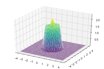
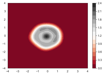
Now get the electron density
fig = plt.figure()
ax = fig.gca(projection='3d')
ax.plot_trisurf(xflat,yflat,get_nxy(num_electrons, psi, x, y),cmap=plt.cm.viridis, linewidth=0.2)
plt.show()
plt.contourf(x, y, get_nxy(num_electrons, psi, x, y).reshape(n_grid,n_grid), 20, cmap='RdGy')
plt.colorbar()
plt.show()
plt.plot(x,nxy.reshape(n_grid, n_grid)[:,n_grid//2])
plt.plot(x,get_nxy(num_electrons, psi_harm, x, y).reshape(n_grid, n_grid)[:,n_grid//2])
plt.xlabel('x coordinate')
plt.ylabel('electron density')
plt.title('cross section of 2D electron density at y = 0')
plt.legend(('with elec-elec interaction','no interaction'),loc='upper right')
print(energy[0:10])
[1.17029678 2.5939502  2.6092069  4.26769901 4.37000567 4.71031507
 6.2792591  6.35870905 7.1566507  7.25873633]
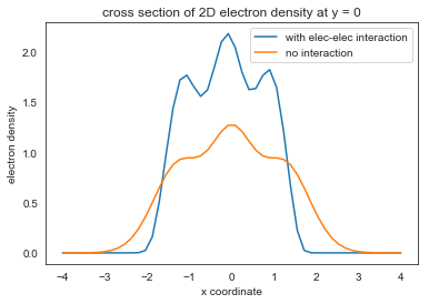
We can see that the electron density actually gets more compact. The elec-elec repulsion just cause the total energy increase. The repulsion effect on density is actually been reversed by elec-elec exchange, which is attractive (in the equation there is a negative sign)